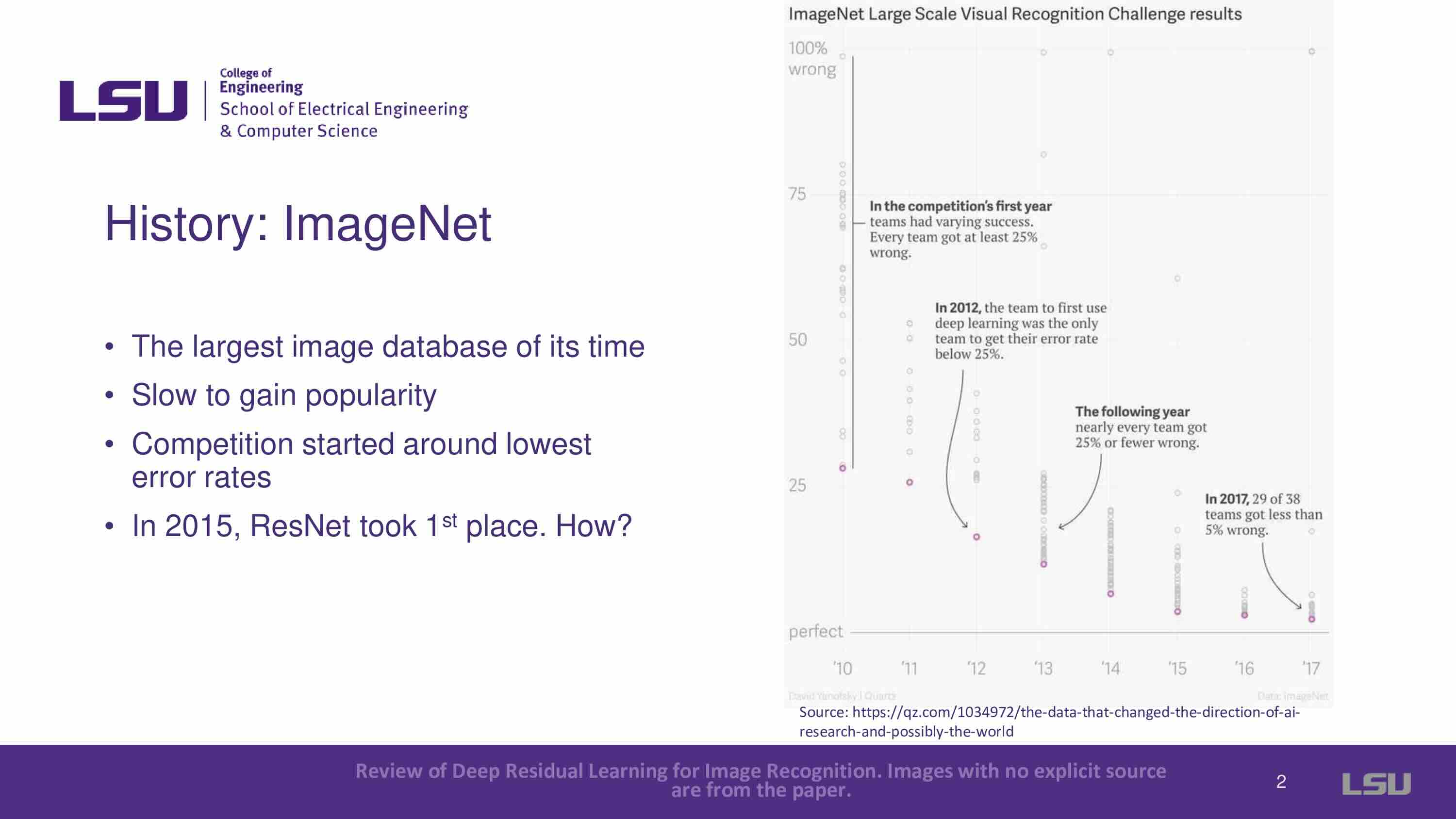
ResNets (Residual Networks) is introduced, and it is mentioned that ResNets won the 2015 ImageNet Large Scale Visual Recognition Challenge. People's curiosity about how they accomplished this led to the publication of the paper in December 2015.
Authors: Kaiming He, Xiangyu Zhang, Shaoqing Ren, Jian Sun
For class EE/CSC 7700 ML for CPS
Instructor: Dr. Xugui Zhou
Presentation by Group 1: Joshua McCain (Presenter), Lauren Bristol, Joshua Rovira
Summarized by Group 6: Yunpeng Han, Yuhong Wang, Pranav Pothapragada
Time: Monday, September 9, 2024
As the number of layers of neural networks increases, the problems of overfitting, gradient vanishing, and gradient explosion often occur, so this article came into being. In this paper, the concept of deep residual networks (ResNets) is proposed. By introducing "shortcut connections," this study solves the problem of gradient vanishing in deep network training and has an important impact on the field of deep learning. The method of the paper explicitly redefines the network layers as learning residual functions relative to the inputs. By learning residuals, the network can be optimized more easily and can train deeper models more efficiently. Therefore, this method can help solve the performance degradation problem that may occur when the network layer increases. In addition, the article displays the experimental part. The model shows significant improvements in handling large-scale visual recognition tasks like ImageNet and CIFAR-10. The application of deep residual networks in major visual recognition competitions like ILSVRC and COCO 2015 further proves their power and wide applicability.
ResNets (Residual Networks) is introduced, and it is mentioned that ResNets won the 2015 ImageNet Large Scale Visual Recognition Challenge. People's curiosity about how they accomplished this led to the publication of the paper in December 2015.
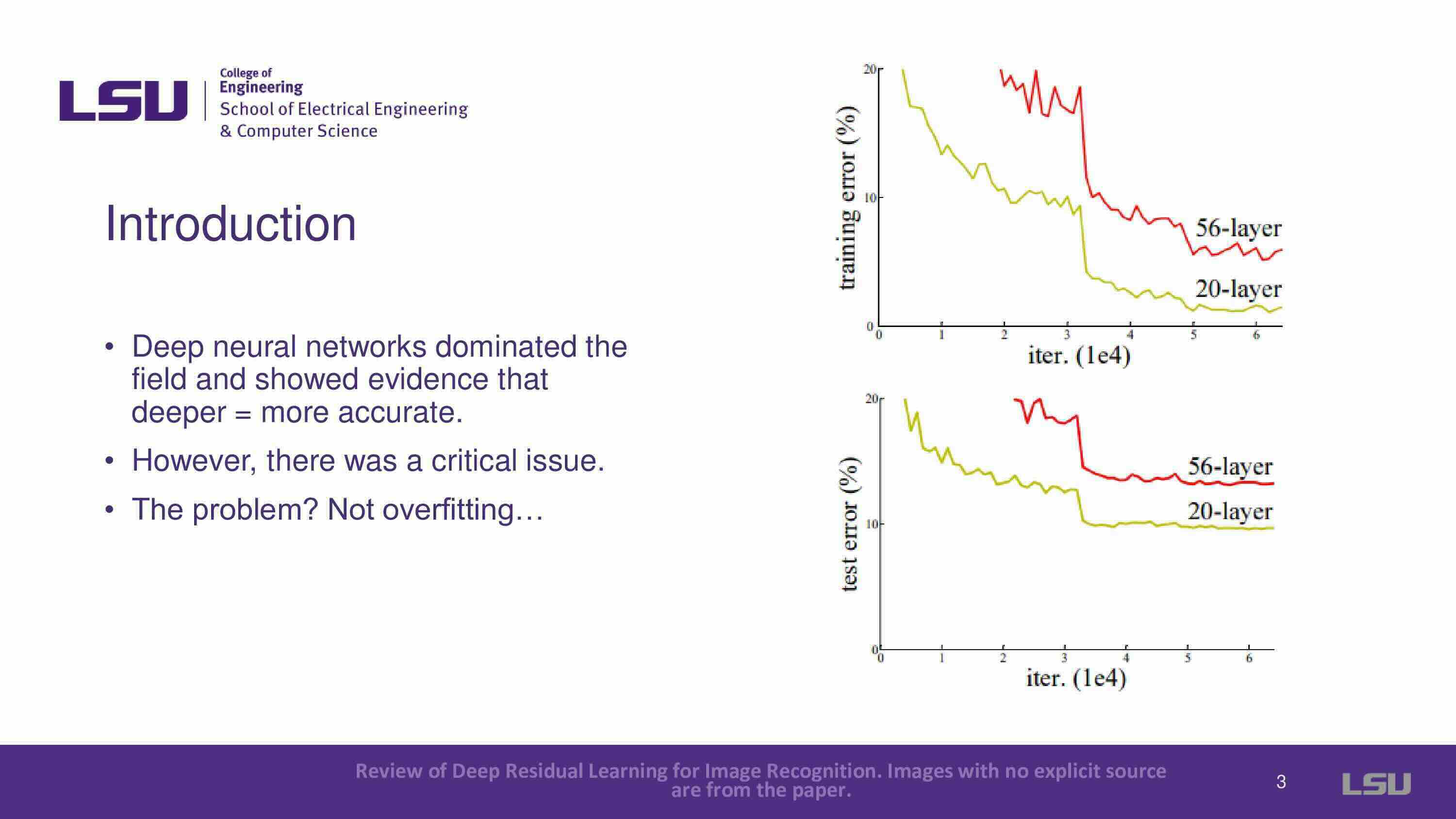
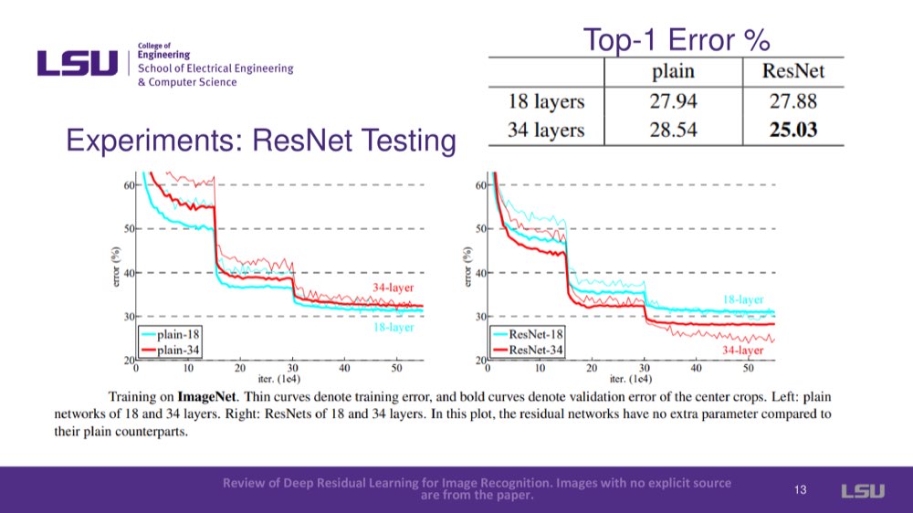
In ML, deeper networks are known to yield more accuracy in machine learning. But a crucial problem surfaced: performance wasn't always enhanced by deeper networks. Contrary to the expectation of overfitting, the 56-layer network performs significantly worse than the 20-layer network, as demonstrated in the slides.
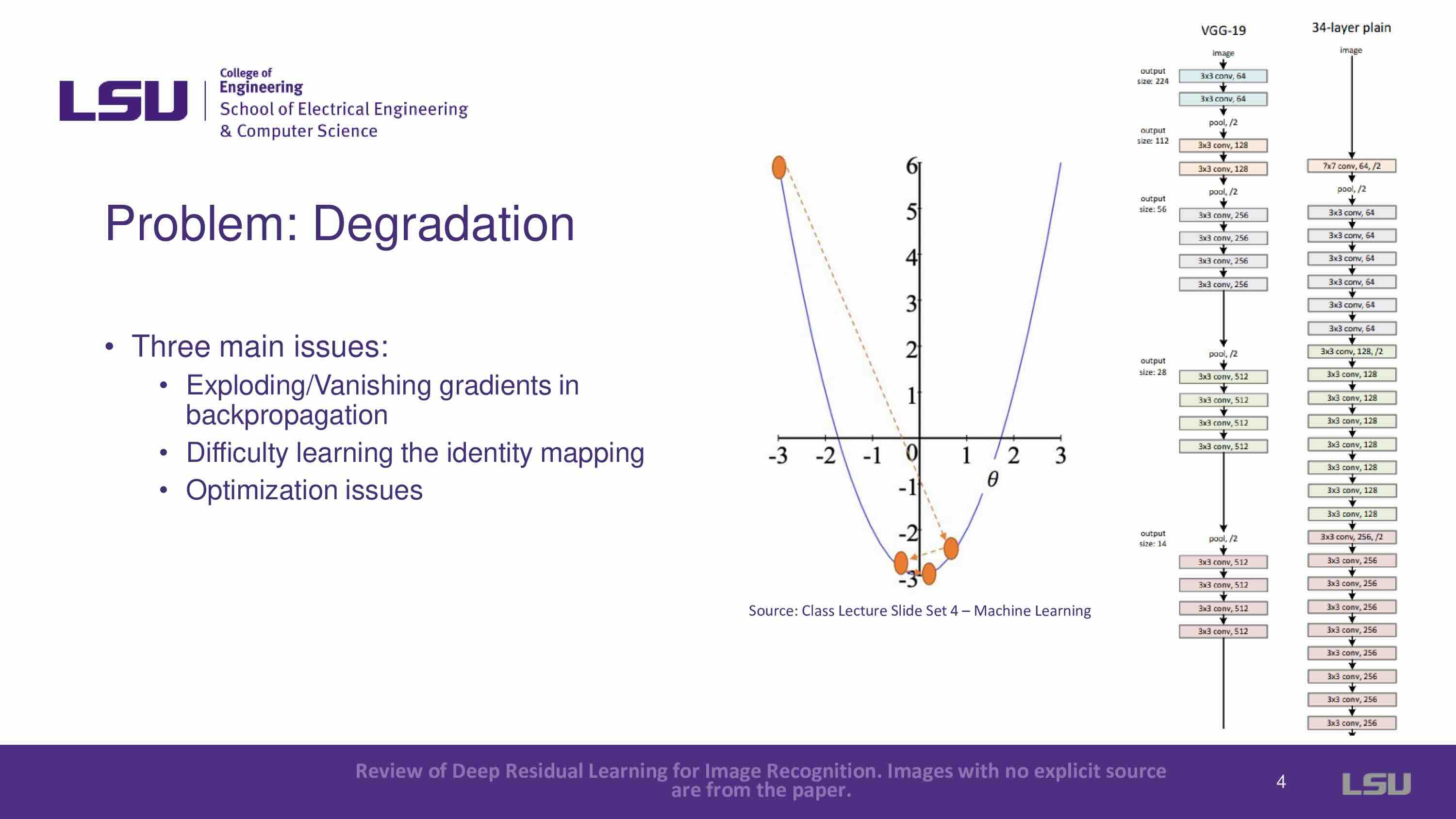
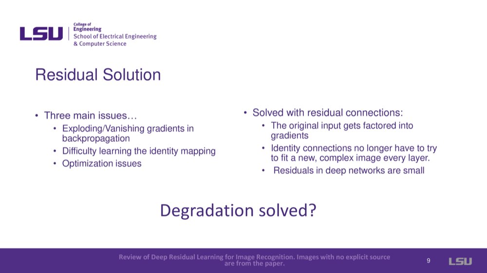
The problem of degradation in deeper networks was addressed. Three main issues with degradation were introduced: exploding/vanishing gradients in backpropagation, difficulty learning the identity mapping, and optimization issues. For vanishing gradients, deeper layers had no reference to the original input. Therefore, it is difficult to adjust weights, especially in deeper networks, and will lead to exploding or vanishing gradients that caused networks to either not converge or get stuck in local minima. For the second problem, difficulty learning identity mapping, the expectation was that a deeper network could map identity (the output should match the input), but this wasn’t the case, and deeper networks failed to maintain accuracy. The third problem is optimization complexity. Each layer in traditional networks had to create a completely new function for every input, increasing the complexity and number of parameters unnecessarily.
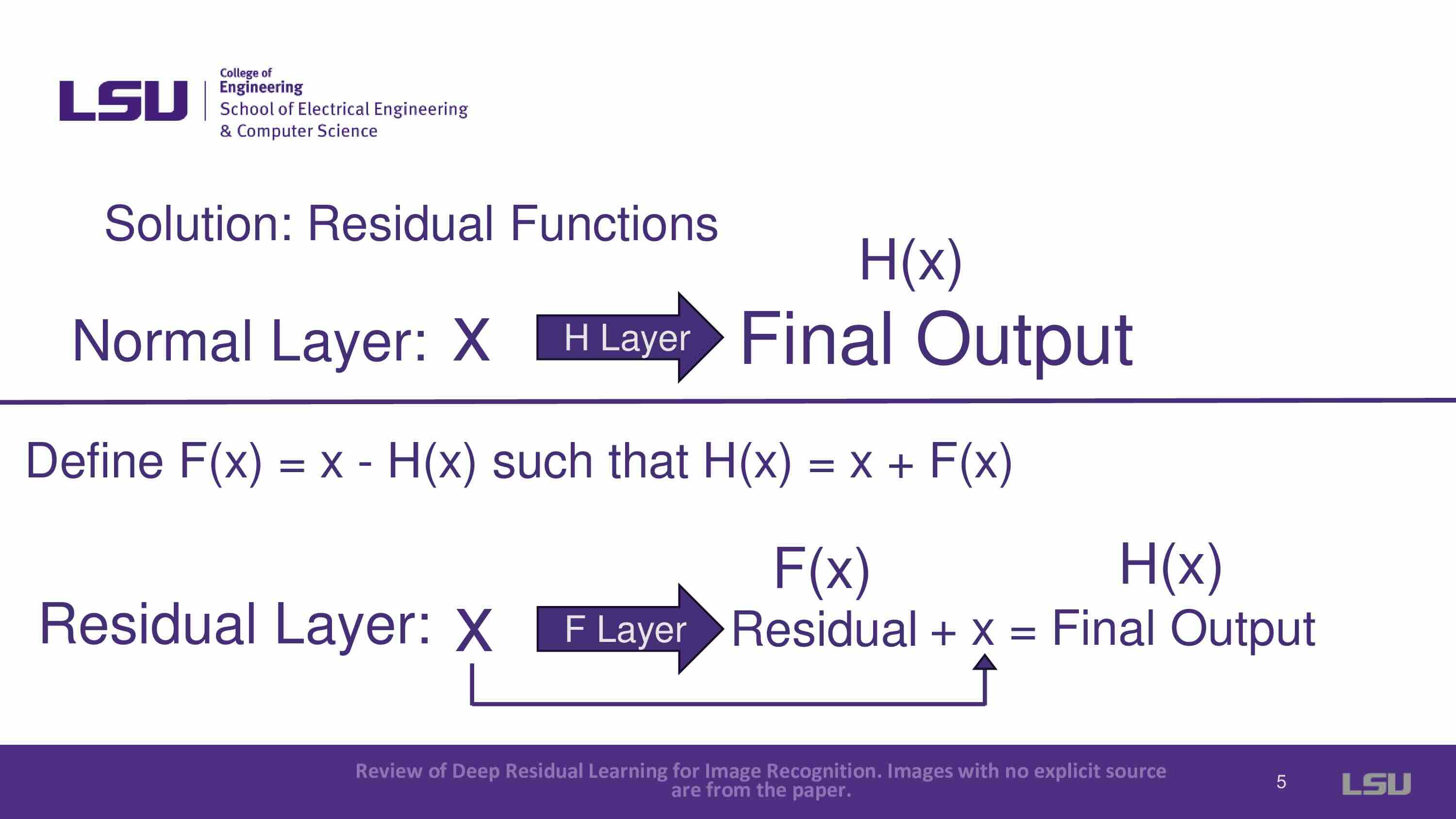
Introduces the concept of residual functions, where instead of trying to map new complex functions in each layer, the residual connection focuses on learning the difference (residual) between input and output and adds that to the input. Formulation: X + F(x) = H(x) where X is input, F means residual layer, F(x) means what after Residual, H(x) means output.
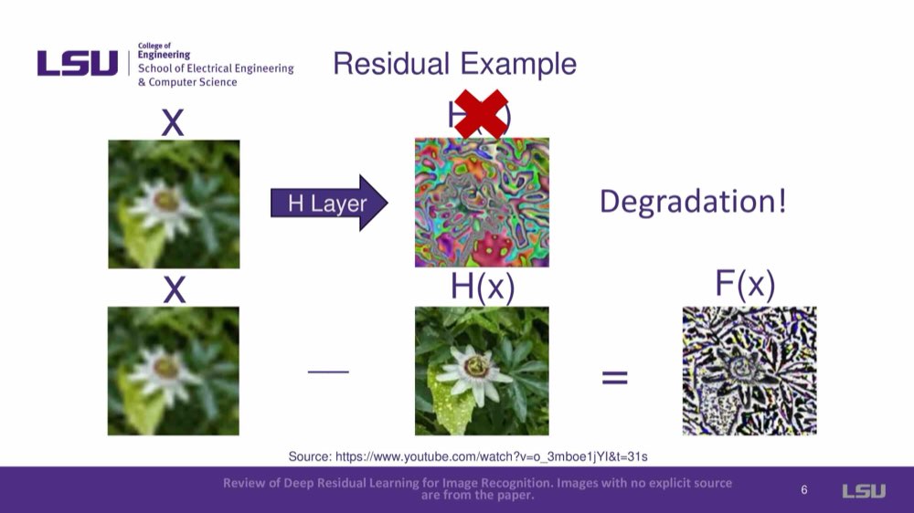
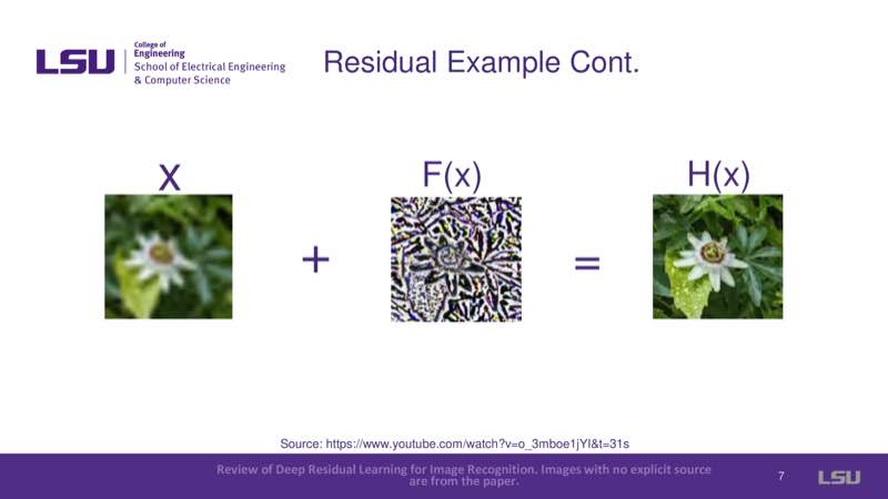
Provides a visual representation of residual functions: X + F(x) = H(x), where x is a blurred image, F(x) is a residual layer, and H(x) is the output image, which is very clear.
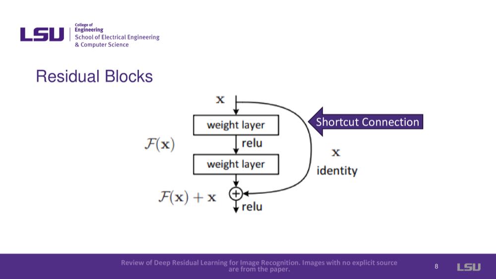
This part shows how the input is carried through a shortcut and added to the residual function to produce the output, solving the degradation problem.
It shows ResNets has some advantages:
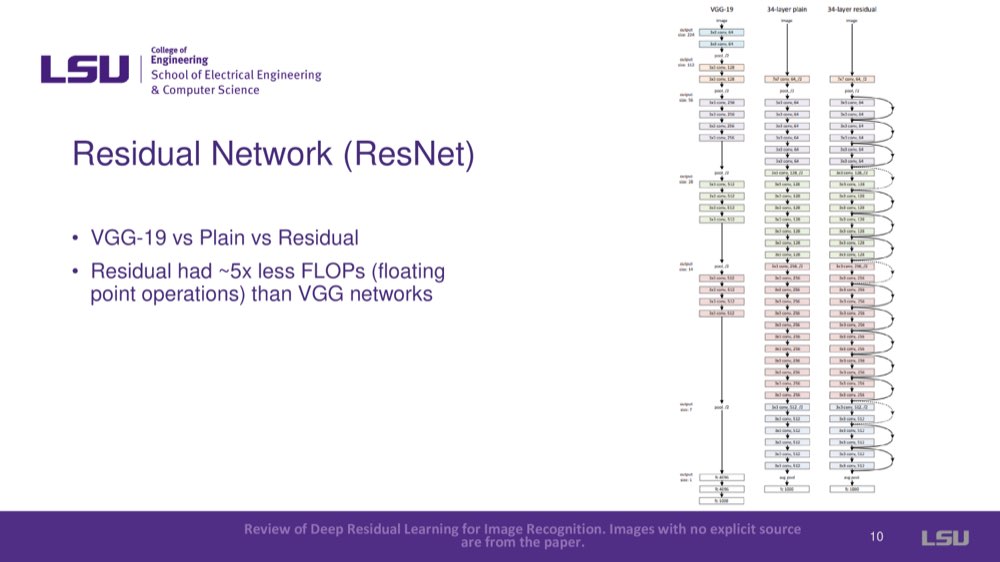
VGG-19, 34-layer Plain, and 34-layer Residual were compared. Residual shows it had ~5x less FLOPs (floating point operations) than VGG networks.
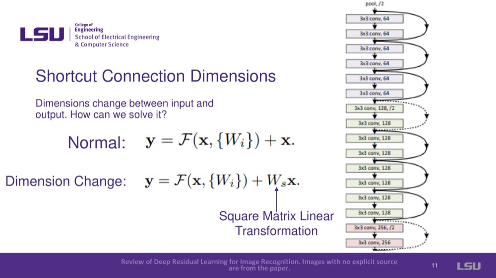
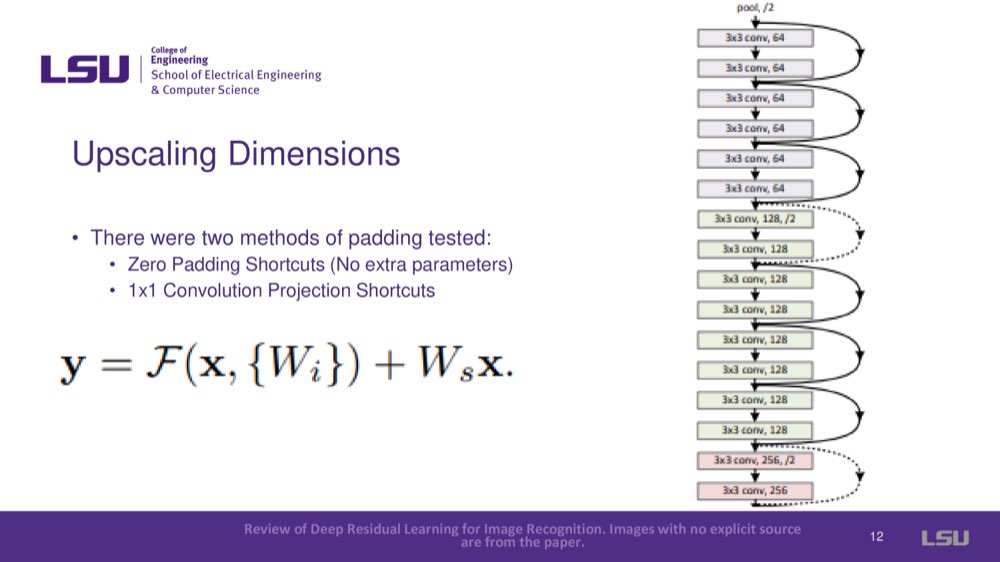
Dimensions change between input and output. How can we solve it? By adding a Square Matrix Linear Transformation, the dimension will change. For upscaling dimensions, there were two methods of padding tested. The first method is the zero having shortcuts (No extra parameters). The other is 1x1 Convolution Projection Shortcuts.
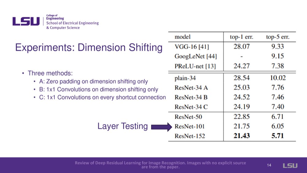
There are three methods that can do dimension shifting: Zero padding on dimension shifting only, 1x1 Convolutions on dimension shifting only, and 1x1 Convolutions on every shortcut connection. The ResNets team tested the network on different datasets to verify its effectiveness. ResNets improved top 1 and top 5 error rates, showing it could generalize well to new datasets.
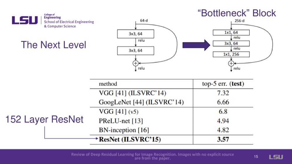
The bottleneck block was introduced, which helped ResNets reach 152 layers while maintaining performance and reducing training time by resizing images inside blocks.
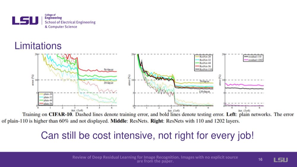
While ResNets solved many drawbacks, deeper networks beyond 1000 layers showed overfitting, indicating limitations in scaling depth indefinitely. ResNets was also computationally intensive and not ideal for every task.
Residual networks can solve the degradation problem through these shortcut connections, which allow networks to go deeper while improving accuracy and reducing the number of parameters required. ResNets did so with fewer parameters than everyone else.
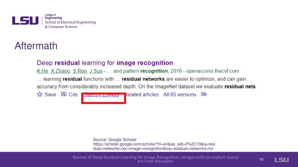
This paper was very influential and cited over 230k times in Google Scholar, which is a foundational paper in machine learning.
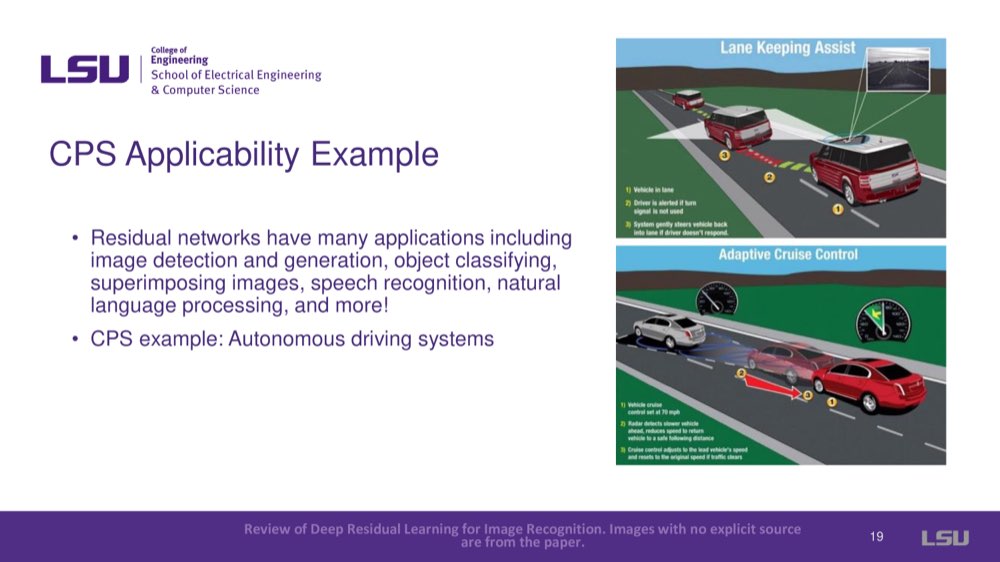
ResNets has broad applications, including autonomous driving systems where accuracy is crucial for tasks like object detection and classification. For example, image detection of stop signs or a car is crucial.
The presenter acknowledges the contributions of teammates who helped with research, examples, and questions.
The idea behind ResNets is to add the input to the output of a set of layers while the layers train to only compute the difference. However, given that the dimensionality of the input is not necessarily the same as the output, we use 1x1 convolutions to extend dimensionality. Other methods of extending, such as zero padding, have also been tested. Still, only performing convolutions on layers that need it seems to strike the right balance between computational complexity and model accuracy.
While it is intuitive to think of it as gradients flowing through the shortcuts presented in the network, it is more accurate to say that the input itself is factored into the gradient. Since the residuals are generally small, we can better avoid vanishing or exploding gradients during backpropagation.
ResNets indeed introduce additional computational complexity and overhead, which is potentially an issue for certain systems. For smaller datasets and less complex applications where very high accuracy is not needed, using ResNets might be overkill and not worth the tradeoff. But when it comes to systems that require accuracy, such as autonomous driving, this might not be that big of an issue, given that while ResNets take slightly more time, they are still fast enough to make real-time decisions without dangerous delays (given a powerful enough computer). In short, it's about balancing speed and accuracy based on importance.
In the ResNet, the network doesn’t subtract the final (required) output from X as is mentioned in the slides; it was an illustration to show how the residuals came into the picture. Instead of generating the necessary input H(x) and subtracting from x to get the residual F(x), the system directly learns to generate the residual F(x), which is generally smaller and hence eliminates the issues presented by generating H(x) directly.
The presenter wrapped up the discussion by pointing out that although robotics wasn’t mentioned much during the conversation, ResNets are relevant in that domain. Like the popular dog robots, robots need sophisticated vision systems to detect and interact with their surroundings. Additionally, for most applications, the number of layers in ResNet models seems to max out at 152, with fewer layers used for less complex tasks.